HOOPS Stream File Exporter

Exporting HOOPS HSF Files

This export converter saves out the database to the HOOPS Stream File (.hsf) file format. The HOOPS Stream File (HSF) file format allows highly compressed files containing 3D data and bitmap images to be streamed over Internet connections of any bandwidth.

Exported entities includes mesh, polyline and trimmed NURBS geometry, object/light/camera/material animation data, materials with embedded texture maps, lights, cameras and a plethora of options to output highly optimized files.

Please also refer to the corresponding Okino HOOPS import converter.

Okino's Overview of the HSF 3D File Format

The HOOPS Stream File (HSF) format is a robust, customizable and highly compressed 2D/3D visualization format specifically tailored to the needs of displaying 3D model and scene data.

Many people in the 3D industry tend to not be familiar with HOOPS, nor have heard of it before. However, HOOPS is one of the oldest and most advanced technologies which still exists today. HOOPS has a long history, starting in the 1980's by Cornell University and then Ithaca Software, followed by Autodesk and finally Tech Soft 3D who are the current developers of the software.

For those "shopping around" for a HSF exporter, keep in mind that Okino was the very first and still primary provider of a HSF file conversion system. We have been involved with HSF from well before it was used elsewhere in the 3D industry and know of the technical particulars of the file format better than anyone. Of particular importance, we do not use any HSF file format SDKs from third party vendors to blindly write out the files. Rather, we have developed our own HSF exporter from the ground up (as is our defacto policy for all Okino exporters) so that we have complete control over the process, and are not at the mercy of any problems from third party SDKs.

HOOPS is the 3D file format used within Autodesk's very popular DWF-3D container file format and the 3D file format used by SolidWorks in their eDrawings container file format. Exporting to the HOOPS HSF format is primarily a process only needed by MotoSim users (please do not use .3ds format to import 3D models into MotoSim, but only HSF format).

Recommendation: if you do not wish to use HOOPS HSF format, then opt to export as DWF-3D files using Okino's DWF-3D exporter and use the extensive Autodesk WEB and desktop DWF-3D file viewers.

Online Scene Demos (HSF Files Exported by PolyTrans). Click any image

Documentation for each HSF Exporter Option Panel

Click on any one of the small screen snapshots to jump to the corresponding section of this WEB page:

Publishing	Compression

Enables	Materials

Curve Output	Mesh Processing

Animation

Advantages of Publishing to the HSF Web Streaming File Format

• No charge for displaying the HSF files on your WEB site. Some other WEB streaming file formats require broadcast license fees or fees to be paid for the publishing package.
  
  
• Free HSF viewer control for WEB browsers.
  
  
• No WEB server configuration required. HSF streaming and viewing is a client-only solution, eliminating the need to endure the considerable IT burden of server-side configuration and maintenance. Users wishing to implement real time collaborative viewing or view-dependent streaming should refer to the HOOPS Net Server.
  
  
• Multiple levels of data compression: vertex, normals, polygon and file-level.
  
  
• Level of Detail support. Streams simpler models first, then successively more complex models.

What types of data is HSF appropriate for?

The HSF format is appropriate for visualization at all phases of the design - manufacture - commerce process chain including CAD/CAM/CAE and related downstream applications all of the way through to e-commerce.

What types of applications can use the HSF format?

HSF is useful for applications in the domains of design, analysis, digital mock-up, machining, view & mark-up, and e-commerce. HSF allows for the same visualization format to be used through all phases of the "art-to-part" process and all of the way through to point-of sale. This flexibility is critical given the trend toward "mass customization" where supplier and customer involvement is occurring further and further up the design process chain and, as such, the line where "e-commerce" begins continues to blur. What this trend reveals is that there should not be a separate format for visualization during the design, analysis and manufacturing phases and another at the point of e-commerce. There is no longer a firm wall between those domains and customers continue to require more sophisticated information about the product. HSF will handle the detailed needs of engineering as well as the lighter weights required for viewing at the point of purchase or during product marketing.

Publishing Options

Flip "Y-Up" to "Z-Up" coordinate system

This option allows the default coordinate system to be set for the output file. It defines what will be considered the "Up" axis in the exported file.

Enabling this option will flip the source Y-up data of the internal Okino scene graph to the Z-up coordinate system of the exported file.

If you find that the data is oriented incorrectly after export then toggle this checkbox.

Report statistics about exported data

If this checkbox is checkmarked then statistics will be output after the file has been exported, which looks similar to:

Number of meshes = 162 Number of polygons = 29319 Number of mesh vertices = 17133 Number of vertex normals = 17133 Number of animated elements = 57 Number of animated instances = 57 Number of lights = 2 Number of directional lights = 2 Number of perspective cameras = 4 Number of orthographic cameras = 5 Number of materials = 42

Publishing and Previewing

Output HTML file with embedded ActiveX viewer

Enabling this option creates an HTML page with the selected file embedded as a file reference. These HTML pages can then be posted to a web site as live 3D data. The HTML page will also contain the necessary code to download the file viewer which will stream the file from either a local disk or a web site into the WEB page for viewing. The embedded object will, behind the scenes, download and install the ActiveX Control if it is not already installed on the machine reading the web page. This means that you simply need to put the HTML and exported file on a Web site and any user of Microsoft Internet Explorer can view the model over the web by simply pointing their browser to the page's URL.

The size of the ActiveX control is specified by the two type-in values, which are specified as a percentage of the HTML page size (1% to 100%).

Preview in WEB browser when done

Enabling this option will cause the exported file to be previewed in the current viewer installed on your machine which recognizes the export file format's file extension.

Published Edges (DWF export only)

Export lines as "Published Edges"
Export NURBs curves as "Published Edges"

These two checkboxes ultimately allow line/curves to be "tagged as published" so that they can be easily hidden or made visible in external Autodesk DWF-3D file viewers.

The DWF file format allows lines and/or NURBS curves to be tagged as being published. This is a simple flag which can be set on such exported line/curve geometry. If either of these checkboxes are enabled then the corresponding geometry type (lines or NURBS curves) will be tagged as "published" in the exported DWF file.

This flagged geometry can be differentiated in downstream DWF file viewers, such as an Autodesk file DWF viewer where the rendering mode can be toggled between Edges Only, Shaded and Shaded with Edges. The lines/curves which have been exported with this Published edges flag set will be hidden in Shaded mode but appear in Shaded with Edges rendering mode of the DWF viewer. These rendering modes can be changed in Autodesk DWF viewers by clicking on the icon which looks like a shaded box with a down arrow beside it - a pop-up menu will appear when you click the down arrow, from which you can choose one of these 3 rendering modes.

As an example of usage, SketchUp files imported using the Okino SketchUp importer usually have both 3D polygon geometry and 3D polyline outlines around the geometrical objects. By enabling this "published" checkbox, the exported SketchUp files to DWF-3D will allow the 3D polyline outlines to be hidden or made visible via the DWF file viewer options mentioned in the last paragraph.

Scene Scaling

Normally the current internal scene should not need any scaling (larger or smaller) before being exported to a destination 3D viewer. However, the following options are available to apply any level of global scaling to all data in the scene, should such scaling be needed. The scaling is applied directly to the coordinate data and any transformation matrices.

Apply global scaling factor

This option allows the exported scene to be scaled larger or smaller by a user specified amount. As examples, enter these values:

1.0, no scene scaling 1000, scale 1000 times larger 0.001, scale 1000 times smaller 4, scale 4 times larger 0.25, scale 4 times smaller

You can enter a value into the edit box specifying a relative scaling factor, and the model will be scaled by this factor. For example, if you enter '2.0', the model will come out twice as large.

Scale exported data to these units

This combo box enables an automatic units matching capability of this exporter. Normally you would not want to use it, especially since you have the manual Apply global scaling factor type-in value above.

The internal Okino scene graph (which is being exported) has an explicit CAD "units of measure" associated with it (editable from the Edit/Preferences/Start-up dialog box in the Okino stand-alone software). This is a purely virtual set of units, not used for anything other than assigning some kind of "unit of measure" to the current scene data. This combo box allows the exported scene to be re-scaled into another virtual set of units. So, if the internal scene units are presently set to "meters" and you set this combo box to "Scale scene to centimeters", then the exported data will be scaled 100 times larger.

Use current scene units (no scaling)

If this combo box option is chosen then no scaling is done and the exported data is not affected by this combo box option at all.

Scale scene to inches
Scale scene to feet
Scale scene to millimeters
Scale scene to centimeters
Scale scene to meters

If the current internal Okino scene units is not the same as the chosen units on this combo box then the exported geometry will be scaled larger or smaller so that the units will match.

Compression Options

Loss-Less Compression Related Options

These checkboxes allow for the exported file to be compressed smaller in size without any loss in quality.

Enable LZ compression on entire file

This enables global compression on the entire file using the "zlib" lossless compression algorithm. It should always be enabled since zlib compression is fairly efficient and fast.

Enable polygon connectivity compression

This compresses mesh geometry connectivity information.  This compression technique can provide compelling reductions in files sizes for datasets that contain many mesh primitives, but can also be a computationally intensive algorithm depending on the size of individual meshes.  You will need to decide for yourself whether the reduced file size is worth the extra computation time.  

Lossy Compression Related Options

This exporter provides sophisticated geometry-specific lossy compression: vertices, normals, uv coordinates and vertex connectivity information. Vertices, vertex normals and vertex texture coordinates are written out with a compact, low resolution format rather than with the original floating-point representation. A variety of compression options can be set in order to balance the reduction in file size vs. the potential increase in export time. Lossy compression means that some quality degradation is to be expected.

Compress Vertices

This compression technique involves encoding the locations of mesh vertices, providing reduction in file size in exchange for loss of coordinate precision and slightly lower visual quality. The degradation in visual quality is highly dependent on the topology of the mesh, as well as how the normals information is being exported.  

Selecting a lower number from the "Bits Per Vertex" drop-down box will cause the file to become smaller but at the expense of lower quality and imprecise vertex locations.

Compress Normals

Enabling this option will cause a degraded series of vertex normals to be streamed in the file. Selecting a lower number from the "Bits Per Normal" drop-down box will cause the file to become smaller but at the expense of lower quality and imprecise vertex normals. Compressed vertex normals will cause faceting artifacts in areas of the model which are highly curved. If the model is not smooth or highly curved to start with then you could use a lower number of bits and still achieve good visual results.

Vertex normals are attributes of each mesh polygon that defines the overall curvature and resulting rendered smoothness of the object. They can consume a sizeable amount of steaming bandwidth and thus compression is desirable for them.

Compress Parameters

This compression technique involves encoding the locations of mesh uv texture coordinates, providing reduction in file size in exchange for loss of coordinate precision and slightly lower visual quality. 

Selecting a lower number from the "Bits Per Parameter" drop-down box will cause the file to become smaller but at the expense of lower quality and imprecise vertex uv texture coordinate locations.

Level of Detail (LOD) Generation

A very important aspect of streaming 3D files across network connections is the time taken to download and display an initial view of the 3D scene to the viewer. For larger models this time can be considerable. To compensate for this long download time "Level of Details" (LODs) can be used. LODs are lower resolution, smaller versions of the mesh models which stream down and display first before the final full resolution mesh arrives. The default exporter options will cause 2 smaller LOD models to be created first in the 3D file before the full resolution model is embedded.

Number of 'Levels of Details' (0 or more):

This determines how many LOD models will be created for the 3D file. 0 will create none. The default is 2.

Decimation amount

This slider determines how much each successive LOD model will be reduced in size. By default this value is 75%. Thus, the first model will be reduced to 75% of the full resolution mesh. The second model will be reduced to (75% x 75% = 56%). The LODs will stream in reverse order, such that the 56% compressed model comes first, the 75% model second and the non-decimated model last.

Decimation algorithm: Fast or Better

This determines which of the mesh decimation algorithms will be used: either the faster (but less appeasing) or better (slow but better more appeasing).

Enables Panel

This panel controls the output of specific geometric mesh attributes, lights and cameras.

Mesh Data Export Options

The basic primitive used to define 3D models in the file are "polygon meshes". The following are attributes associated with the output of the mesh data.

Output vertex normals

If this checkbox is checkmarked then vertex normals will be exported along with the mesh geometry. Vertex normals are used to specify where an object is to appear smooth and where it is to appear faceted (rough).

Output u,v texture map coordinates

If this checkbox is checkmarked then (u,v) vertex texture coordinates will be exported along with the mesh geometry. uv texture coordinates are used to define how a bitmap texture image is to drape over and around a mesh model.

Output vertex colors (if available)

If this checkbox is checkmarked then all of the colors assigned to each and every vertex will be exported along with the mesh geometry. Vertex colors are rare or non-existent for CAD data, but rather they are often used in 3D game development instead of explicit materials to define the color and shading characteristics of a mesh's appearance.

Want convex polygons only

Checkmark this checkbox to cause non-convex (concave) polygons to become triangulated. An example of a concave polygon is a "star shape".

Want quadrilateral polygons only

Checkmark this checkbox to cause 5 or more sided polygons to become triangulated.

Want triangles only

Checkmark this checkbox to cause 4 or more sided polygons to become triangulated. This is the default option simply because it has been seen that some file viewers do not display files properly which have 4-sided quad polygons. There is no reason you can't disable this option and output quad polygons.

Output point sets

If this checkbox is checkmarked then 3D point set geometry will be output. 'Points' are 1 or more 3D points in space, with no area or line length.

Output lines and polylines

If this checkbox is checkmarked then 3D line set geometry will be output.

Output NURBS surfaces (patches)

If this checkbox is checkmarked then trimmed NURBS surfaces will be exported, either in raw form or as converted polygon meshes.

Note: NURBS surface cannot be textured since they do not have explicit uv texture coordinates. In such cases keep the Output NURBS as polygon meshes option enabled so that proper uv texture coordinates get exported along with the tessellated meshed version of the NURBS surface.

Output NURBS as polygon meshes

If this checkbox is checkmarked then the raw trimmed NURBS will be tessellated into a polygon mesh prior to export. If it remains uncheckmarked then the raw trimmed NURBS data will be exported directly.

Output NURBS trim curves

If the above option is disabled (pure NURBS output enabled) then this checkbox determines whether trim curves will be output along with the parent trimmed NURBS surfaces. Trim curves define the outer boundary of a NURBS patch as well as specifying internal trim holes and islands.

Output Cameras, Type = TKE_Camera, TKE_View

This combo box determines which camera opcode definition will be exported. Basically, both are identical. The preference is to the 'TKE_View' opcode. Both are provided in case some destination viewer prefers one camera opcode type over another.

Output meta-data information

Enabling this option will output meta data items associated with instances, objects, lights and cameras of the current internal scene graph.

The following internal Okino scene graph meta data types are supported during the export process: strings, shorts, ints, floats, colors, vectors, double precision vectors, 4x4 matrices, 4x4 double precision matrices, time, double precision floats, 4 valued vectors, and 4-valued double precision vectors. All numeric values will be converted into meta data string for output.

Materials Panel

This panel controls the output of materials and texture definitions.

Output materials ('surface' definitions)

If this checkbox is checkmarked then the following material attributes will be exported:

• Diffuse surface color.
• Specular highlight color.
• Face opacity.
• Phong highlight size.
• Reflection coefficient.
• And optionally the first diffuse texture map.
• (there is no capability in the 3D file to accept an ambient color)

Embed Texture Images, max size = ( 16 to 8192 )

If this checkbox is enabled then the first diffuse texture map assigned to the material will have its bitmap image read from disk and embedded directly inside the file. This will require that the "uv texture coordinates" mesh option be enabled as well.

The combo box specifies the maximum resolution of bitmap image which is allowed to be embedded in the exported file. For example, if the combo box is set to 256, but the source bitmap image is 1024x1024 in size, then the image will be scaled down to 256x256 pixels in size prior to embedding in the exported file.

Force HSF style texture (DWF output only)

Normally you would want to keep this checkbox disabled. We consider this a 'debugging option' whereby it is easier for us to extract any embedded texture maps using this method. However, it may have other uses to users of this exporter.

The DWF file format is actually a 'container format', a ZIP file archive of many different other files. If this checkbox is disabled (which is the default) then the texture mapping bitmap images will be stored in this ZIP file (the DWF container file) as explicit and individual PNG, TIFF, JPEG, etc. images.

If this checkbox is enabled then the images will be embedded within a HOOPS .hsf file as raw binary image data. The HSF file is the '3D geometry content' portion of the DWF ZIP container archive. In other words, the DWF file will contain a .hsf file for the 3D content, and that one .hsf file will contain all the texture mapping bitmap image files are embedded binary content data.

Output Spherical Environment Maps

If this checkbox is checkmarked then if the material has a spherical environment map associated with it then it'll be exported to the 3D file as a related spherical environment map.

Texture Filtering Method:

This specifies the default texture filtering method for the destination file viewer. When a texture image is blown up much larger or much smaller than its normal dimensions then "texture aliasing" artifacts can appear on the viewed model. To compensate for these aliasing artifacts the viewer program can perform "texture filtering". Multiple methods exist for the exporter. "MIPmaps" and "Summed Area Tables" are common methods.

Enable JPEG Image Compression

If this checkbox is enabled then the texture images embedded within the file will be compressed using JPEG compression. The default is 75. The acceptable values are 1 to 100, with higher numbers resulting in better quality but lower levels of compression.

Shading Coefficient & Colors Overrides

The first two combo boxes and single numeric text box provides hands-on control over how exported material shading parameters should be modified so that the exported model can be rendered nicely as it would have looked in the source 3D program. The two combo boxes and the single numeric text box provide you good control over the ambient, diffuse, specular, luminous, opacity and shininess shading coefficients exported to the file.

The first drop-down combo box selects which of these shading parameters is to be modified. Each shading coefficient has its own operation that can be selected (via the second combo box) and an optional numeric text value (via the third data entry text input box). The following describes the various shading parameters that can be controlled:

Ambient Coefficient: This controls the amount of color reflected from an object based on the ambient light in a scene. A good default value is 0.1 through to 0.3 and ideally ranges from 0.0 to 1.0.

Diffuse Coefficient: This controls the amount of color reflected from an object based on the direct light shining on it. A good default value is 0.4 and ideally ranges from 0.0 to 1.0.

Specular Coefficient: This controls the intensity of the highlight color on an object. A good default value is 0.7 and ideally ranges from 0.0 to 5.0.

Luminous Coefficient: This controls how much color is added directly to an object, regardless of any light that shines on it (the higher the value, the more the object will appear to glow). In general this value should be kept at 0.

Opacity: This is the inverse of transparency. 0.0 will make the object fully transparent, while at 1.0 the object will be fully opaque.

Phong Shininess: This controls the width of the specular highlight seen on an object. An ideal range is 6 (very wide) to 300 (very narrow). The default is 32.

For each material shading parameter, several actions can be performed on each material shading parameter during the import process:

Do Not Export: When this option is selected, the shading parameter is set to 0, effectively making the shading channel appear black (for color channels).

Export Unchanged: When this option is selected, the shading parameter is exported as is, with no change.

Set and Use Default: When this option is selected, the shading parameter is set to some "good" default value (as determined by the export converter). This default value will be displayed in the input text box.

Set to Specific Value: When this option is selected, the exported shading parameter will be overridden with the user specified value of the numeric input text box.

Export and Crop by: When this option is selected, the shading parameter is exported and will remain unchanged if it is less than the numeric text input value shown on the dialog box. If it is greater, then the exported value will be clamped to be no greater than the numeric type-in value. This is a good operation, for example, if you do not wish for the ambient shading coefficient to be greater than 0.3.

Export and Scale by: When this option is selected, the shading parameter is exported and multiplied by the numeric input text value shown on the dialog box

Normalize Color and Coefficient: When this option is selected, this option only applies for the ambient, diffuse, specular and luminous shading coefficients and their respective RGB colors. This option is a hybrid approach that tries to automatically "guess" at a proper shading coefficient value given the raw (and corresponding) color imported from the file. As mentioned earlier, the shading coefficient is needed to create nice looking (nicely shaded) images in a photo-realistic rendering program. If this option is selected, then the specific shading coefficient will be derived directly from the relative intensity of the imported color that corresponds to this shading coefficient (diffuse color for diffuse shading coefficient etc.). For example, if the imported diffuse color is (0.4, 0, 0), which is 40% of full-bright red, then the diffuse shading coefficient will be set to 0.4 and the diffuse color will be modified to be (1, 0, 0). When the new color (1,0,0) and the new shading coefficient (0.4) ar multiplied together, it results in the original color imported from the file (0.4, 0, 0). In general you may wish to use the "Set and Use Default" option to get good rendered results.

Multiply Colours By Material Shading Coefficients

Inside Okino's internal scene graph each material has a "color" and a corresponding "shading coefficient" for each ambient, diffuse, specular and luminous color definition. The "shading coefficient" can be considered a variable intensity control that brightens or darkens its corresponding color, without having to modify the color itself.

If this checkbox is checkmarked then each shading coefficient is multiplied into its corresponding color value before being exported to the 3D file material. Normally you would want this option enabled as it creates a 3D material definition which is very close in appearance to an Okino material definition.

If this checkbox is not checkmarked then only the raw colors will be output (diffuse, specular and luminous) to the 3D file and their corresponding shading coefficient values will be ignored. This will typically result in brighter, bolder and punchier materials, what we ourselves term "OpenGL" shading which tends to be more saturated than colors seen in photo-realistic rendering programs.

Set specular material color to white

If this checkbox is enabled then the specular material color will always be set to white (although, the white can be dimmed by changing the 'Specular Coefficient' material parameter override, as described above). If disabled, then the real material's specular color will be output.

Merge and mix Ambient color into the Diffuse color

The output file format has no capability of accepting the ambient material color. Only the diffuse and specular material colors can be exported and retained. To overcome this problem, enabling this checkbox will cause the material's ambient color to be mixed into the diffuse material color before the final diffuse color is exported. Disabling this checkbox will not output any ambient material color.

Mesh Processing Options Panel

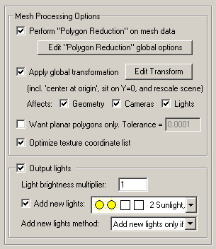
This panel controls the processing options of the polygon mesh exporter "engine".

Perform "Polygon Reduction" on Mesh Data

If this checkbox is enabled (check-marked) then the exporter will apply the global polygon reduction algorithm to each mesh object just prior to them being embedded in the file.

The algorithm allows the number of polygons in the scene to be greatly reduced. The parameters used to reduce the polygons can be modified by pressing the "Edit Polygon Reduction Global Options" button. Press the "Help" button on its corresponding dialog box to learn more about the polygon reduction system.

Apply global transformation

If this checkbox is enabled then a general purpose global transformation will be applied to each exported scene. This new transformation matrix will be applied to the root node in the exported file.

This option will allow you to, for example,

• Re-center all of the geometry so that it is centered at the origin (0,0,0) in the file.
• Move all of the geometry so that it is sitting on the Y=0 (XZ) horizontal plane.
• Auto-scale the geometry so that it is no larger than a specific bounding box size.
• Scale the scene by a (X, Y, Z) value.
• Shear the scene by a (X, Y, Z) value.
• Rotate the scene by a (X, Y, Z) value.
• Translate the scene by a (X, Y, Z) value.

Since the lights and cameras are attached to this new global transformation node, they will be affected along with the geometry.

The transformation can be edited by pressing the "Edit Transform" button which will cause the following global transformation dialog box to appear:

The transformation matrix will be computed in two phase: (1) the transformations specified in the top "Automatic Scene Resizing" section, then (2) the single transformation specified in the "General Transformation Matrix" section.

The values on the dialog box are described as follows:

Automatic Scene Resizing

Center all geometry at the origin

If this checkbox is enabled (checkmarked) then all the geometry data will be positioned so that it is centered about the origin. If disabled then the geometry will not be repositioned.

Make all geometry sit on the Y=0 horizontal plane

If this checkbox is enabled (checkmarked) then the geometry will be repositioned so that it is sitting flush with the top of the Y plane (the horizontal plane).

Scale geometry to be no larger than:

This option allows the geometry data to be automatically rescaled if it is too large. If set to 'Do not scale the geometry' then no scaling will be done. If set to '1x1x1 units' then all the objects will be scaled smaller should they exceed 1x1x1 units in total size. Likewise for the '2x2x2 units' option. If set to 'User defined maximum size' then the maximum size of all the objects can be set using the type-in numeric box. The default is '2x2x2 units'.

Although not quite the same, if the option is set to 'Use Absolute Scaling Factor' then all objects exported to the file will be scaled absolutely by the user specified value. Thus, if you set the type-in value to 0.25 then all objects will be made 4 times smaller and if the value if set to 4 then all objects will be scaled 4 times larger. This is useful is you are converting a variety of different models to the export format and you want them all uniformly scaled with the same scaling factor.

Transformation Matrix Values

Translate X, Y, Z

This applies a 3D translation by the specified amounts in the X, Y and Z dimensions.

Scale X, Y, Z

This applies 3D scaling in the X, Y and Z dimensions. All 3 scale factors must be non-zero. Values above 1.0 will make the scene larger (2.0 will double the size of the scene) while values less than 1 will make the scene smaller (0.5 will half the size of the scene).

Shear XY, XZ, YZ

This applies a linear shear in one of 3 directions:

XY will shift all points in the X direction by the specified amount in proportion to the distance the points are located along the positive or negative Y axis. For example, using a value of 2.5 will shear all points by 68 degrees in the positive X direction; in other words, for every unit increase in the Y direction the X points will be shifted by 2.5 units.

XZ will shift all points in the X direction by the specified amount in proportion to the distance the points are located along the positive or negative Z axis.

YZ will shift all points in the Y direction by the specified amount in proportion to the distance the points are located along the positive or negative Z axis.

Rotate Around X Axis
Rotate Around Y Axis
Rotate Around Z Axis

This applies a rotation about the X, Y and/or Z axes. The rotation angle is restricted to the range -360 to 360 degrees. The angle of rotation is counter-clockwise when viewed from the positive to negative axis of rotation.

Output Lights

If this checkbox is checkmarked then all light sources of the current 3D scene will be exported to the file, including those parameters for ambient, point, spot and directional light sources.

Light brightness Multiplier, #

You can enter a light intensity "multiplier" value into this type-in box. Entering 2.0 will output the light intensities double their normal values while a value of 0.5 will output the light intensities at half their normal values.

Add new Lights

If this checkbox is checkmarked then new lights will be added to the export file. The pre-defined light locations, color and light types are chosen from the following drop-down combo box.

• The first two icons represent the light type (Sun = directional light, Light bulb = point light, Spot light = spot).
• The second two squares represent the color of each of these two light sources.
• The text describes the location of the new light sources (see image below for visual locations).

The new light sources will be placed according to the following image, along the XY plane. If you are looking down the Z axis (towards the negative Z axis) then upper-left will be (1), upper-right will be (3), lower-left will be (7) and lower-right will be (9).

Add New Lights Method

This combo box determines how the new lights are to be added to the exported file.

Merge with existing lights in the scene

This option will cause the newly chosen lights (from the drop-down combo box mentioned above) to be added to the already existing lights of the current 3D scene. In other words, all the lights of the current 3D scene will be output first, followed by the 1 or 2 new lights you have chosen from the drop-down visual list.

Replace existing lights in the scene

This option will cause the newly chosen lights (from the drop-down combo box mentioned above) to be output to the export file, but no other light sources. None of the light sources in the original 3D scene will be output to the export file.

Add new lights only if there are no existing lights in the scene

This option will cause the newly chosen lights (from the drop-down combo box mentioned above) to be output to the export file, but only if there are no existing lights in the original 3D scene. This is the default option. It will ensure that there are at least 1 or 2 new light sources added to the exported scene if no lights exist in the original 3D scene.

Curve Output Options Panel

This panel controls the output of 3D NURBS curves, 3D spline shapes and 3D Polyline curves. The output file format accepts either pure NURBS curves or 3D polylines.

Output independent 3D NURBS curves

The internal Okino scene graph has a very extensive NURBS curve sub-system. Each NURBS curve object can have 1 or more NURBS curves associated with it. Multiple curves inside a single object can either be considered to form a single continuous "composite" curve, or each curve can be considered unique, closed, planar (in world space) and oriented such that the curves of the object can be directly converted into a trimmed NURBS surface (in other words, the first curve forms the boundary of the surface and subsequent closed curves form the holes).

The following options control how the various NURBS curve configurations can be converted during the export phase. An extensive internal NURBS curve conversion and cross-conversion system exists.

If 'renderable flag' enabled in NURBS curve primitive:

[No Change]

No change. The NURBS Curve primitive will be exported as-is.

Convert and Output as Polygon Mesh

The NURBS Curve primitive will be converted into a mesh object prior to export.

Convert and Output as Trimmed NURBS Surface

The NURBS Curve primitive will be converted into a corresponding trimmed NURBS surface (patch). If the conversion process cannot be made then it will be output as a polygon mesh instead.

If 'renderable flag' not enabled:

If the 'renderable' flag of a NURBS Curve primitive is not enabled then the curves will be considered just as plain curves that cannot be seen when rendered. In this case, the following options define what will be done to NURBS Curves primitives during the export phase when their 'renderable' flag is disabled:

[No Change]

No change. The NURBS Curve primitive will be exported as-is.

Convert and Output as a Spline Shape

No change except in the case when the NURBS curve primitive is defined as a single composite curve made up of multiple curve segments. In this case the multiple curve segments will be temporarily converted to a single NURBS curve before export.

Convert and Output as a PolyLines

The NURBS Curve primitive will be converted into a similar and corresponding Polyline primitive before export.

Output independent 3D spline shapes

The internal Okino scene graph has a very extensive spline primitive sub-system. This primitive accommodates one or more spline curves per primitive. If the multiple spline curves are each closed then the overall Spline Shape is termed "renderable" and can be thus converted into a polygon mesh or a corresponding trimmed NURBS surface (patch). For example, the letter "B" can be defined by 3 Bezier curves, the first forming the outer boundary and the latter two forming holes. Note, that unlike the NURBS Curve primitive, each spline curve of the Spline Shape is composed of only a single curve segment (no composite spline curves are allowed).

The following options control how the various Spline Shape configurations can be converted during the export phase. An extensive internal Spline Shape conversion and cross-conversion system exists. The Spline Shape primitive also handles almost every major spline type (Bezier Spline, B-Spline, Cardinal Spline, Linear Spline, Tensioned Spline, TCB Spline), and their internal cross conversion (between spline types) or between the various spline types and a NURBS curve.

If 'renderable flag' enabled in spline shape primitive:

Convert and Output as Polygon Mesh

The Spline Shape primitive will be converted into a mesh object prior to export.

Convert and Output as Trimmed NURBS Surface

The Spline Shape primitive will be converted into a corresponding trimmed NURBS surface (patch). If the conversion process cannot be made then it will be output as a polygon mesh instead.

If 'renderable flag' not enabled:

Convert and Output as a NURBS Curve Object

Each spline curve of the Spline Shape primitive is resampled into a corresponding NURBS Curve segment and placed into a single NURBS Curve primitive. The 'renderable' flag of the new NURBS Curve primitive will be disabled. The final NURBS Curve primitive will look similar (within an error tolerance) to the original Spline Shape.

Convert and Output as Polylines

Each spline curve of the Spline Shape primitive is resampled into a corresponding Polyline linear curve.

Animation Options Panel

This panel controls the export "animation conversion engine". This engine allows any form of animation data (TCB, Bezier, Euler, Quaternion, etc) to be cleanly exported.

Output object animation data

If this option is enabled (checkmarked) then animation data associated with an instance (geometry) will be exported. Animation data consists of scale, rotation and translation function curves.

Output camera animation data

If this option is enabled (checkmarked) then animation data associated with a camera will be exported. Animation data consists of look-from, look-at (or quaternion) and field-of-view animation curves.

NOTE: "Look-at, targeted" cameras cannot do camera 'roll' curves around the look- at vector simply because the file format does not support it.

Output light animation data

If this option is enabled (checkmarked) then animation data associated with a light will be exported. Animation data consists of shine-from, quaternion shine direction and light color.

Output material animation data

If this option is enabled (checkmarked) then animation data associated with a material will be exported. Animation data consists of the diffuse color, specular color and opacity.

Camera type:

Free camera (rotation based)

If this radio button is chosen then the camera will be animated by a look-from XYZ vector animation channel and an animated rotation vector. This is similar to the "Free camera" in 3ds Max.

Look-at camera (targeted)

If this radio button is chosen then the camera will be animated by a XYZ look-from vector animation channel and a XXZ look-at vector animation channel. As such, we refer to this as a "targeted" camera, since the camera will look at a specific XYZ location.

NOTES:

• "Free cameras" can suffer from precision playback problems as experienced with Autodesk DWF file viewers. This is due in part to the use of animated quaternions to specify the direction viewing vector.
• "Look-at, targeted" cameras cannot output camera 'roll' animation as it does not exist in the file format.

Output keyframe time values as:

Some basic explanation is needed to understand this set of radio buttons:

• Okino animation keys have time values specified in "tick time". Rather than specify the time of each key in "seconds" or "frames", they are instead specified in units of 1/4800th of a second. This 1/4800th of a second is called "one tick of time".
  
  
• HSF animation is ALWAYS output as "tick time", where each 1 unit of time is equivalent to 1/4800th of a second. The "ticks per second" parameter found in HSF files will be set to 4800. Hence, raw Okino animation key times will be output directly to HSF files unchanged and correct. These two radio buttons are completely ignored while outputting animation data to HSF file.
  
  
• The problem is for Autodesk DWF file viewers. In simple terms, they ignore the "ticks per second" parameter of the file and only allow playback at 3 pre-defined speeds which this exporter cannot control: 3, 10 and 30 "ticks per second". Using more common but equivalent terminology, Autodesk DWF file viewers play back animation from a DWF file at 3, 10 or 30 "frames per second". Using the HSF "4800 ticks per second" would cause the animation to play back at a terribly slow rate in any DWF file viewer. Hence you will want to keep this radio button set to "Frame numbers" to allow for exported animation data which plays back at the fast "30 ticks per second" mode found in DWF file viewers.

"Tick time" (1/4800th of a second)

If this radio button is chosen then each key of an animation channel will have its time specified in "tick time" (1/4800th of a second). In other words, the raw Okino animation frame times will be output to both HSF and DWF files unchanged. This is fine for HSF files.

However, this option is currently not ideal for animation played back in Autodesk DWF file viewers because they want the animation timing to be either 3, 10 or 30 ticks-per-second. Hence the alternative "Frame numbers" radio button should be used.

** In the future, if you acquire a DWF file viewer which can read the "ticks per second" opcode from the file (1/4800th in the case of the Okino exporter), and it does not impose the 3, 10 or 30 ticks-per-second playback speeds, then choose this "Tick time" radio button instead. So, in basic terms, Okino is providing these 2 radio buttons for future cases where a proper DWF file viewer is made available, a file viewer which reads and respects the "ticks per second" opcode from the DWF file.

Frame numbers (at current frame-per-second rate)

In simple terms: choose this radio button when outputting animation which is destined for an Autodesk DWF file viewer which can only play back animation at 3, 10 or 30 "ticks per second". Choose the "30 ticks per second" fast playback mode in the file viewer to be equivalent to the 30 frames per second playback speed of Okino software.

Note: this radio button will be ignored when exporting HSF files, for which the animation frame times will always be output in 1/4800th of a second ("tick time").

Common Animation Resampling Export Options

Pressing this button will show the animation resampling and reduction options dialog box. This, in general, controls the precision and reduction options used globally during animation resampling (for both import and export). If you find that your exported animation data looks jittery or does not hit target translations/rotations, then reduce the tolerance values and/or disable keyframe reduction. To learn more about this dialog box press the "Help" button located on it.